Maurice Clerc (
Maurice.Clerc@WriteMe.com) http://www.mauriceclerc.net29 February 2000
The classical Particle Swarm Optimization is a powerful method to find the minimum of a numerical function, on a continuous definition domain. As some binary versions have already successfully been used, it seems quite natural to try to define a more general frame for a discrete PSO. In order to better understand both the power and the limits of this approach, we examine in details how it can be used to solve the well known Traveling Salesman Problem, which is in principle very "bad" for this kind of optimization heuristic. Results show Discrete PSO is certainly not as powerful as some specific algorithms, but, on the other hand, it can easily be modified for any discrete/combinatorial problem for which we have no good specialized algorithm.
L'Optimisation par essaim particulaire est une méthode efficace pour trouver le minimum d'une fonction numérique définie sur un domaine continu. Certaines versions binaires ayant été déjà utilisées avec succès, il semble assez naturel d'essayer de définir un cadre plus général pour une OEP discrète. Afin de mieux comprendre à la fois l'efficacité et les limites de cette approche, on examine en détail comment elle peut être appliquée au bien connu Problème du voyageur de commerce, qui est, a priori, très "mauvais" pour ce genre d'heuristique d'optimisation. Les résultats montrent que l'OEP discrète n'est sûrement pas aussi performante que certains algorithmes spécifiques, mais, d'un autre côté, elle peut facilement être adaptée à tout problème discret/combinatoire pour lequel on ne disposerait pas de bon algorithme spécialisé.
The basic principles in "classical" PSO are very simple. A set of moving particles (the swarm) is initially "thrown" inside the search space. Each particle has the following features:
From now on, to put b) and c) in a common frame, we consider that the "neighbourhood" of a particle includes this particle itself.
At each time step, the behaviour of a given particle is a compromise between three possible choices:
This compromise is formalized by the following equations:
![]()
Equ. 1. Basic equations in "classical" PSO
with
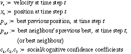
The three social/cognitive coefficients respectively quantify:
Social/cognitive coefficients are usually randomly chosen, at each time step, in given intervals.
Of course, many works have been done to study and to generalize this method . In particular, I use below a "nohope/rehope" technique as defined in , and the convergence criterion proved in .
Also, there are many ways to define a "neighbourhood" , but we can distinguish two classes:
So, what do we really need for using PSO ?
Usually, S is a real space ![]() , and f a numerical continuous function. But in fact, nothing in Equ. 1 says it must be like that. In particular, S may be a finite set of states and f a discrete function, and, as soon as you are able to define the following basic mathematical objects and operations, you can use PSO:
, and f a numerical continuous function. But in fact, nothing in Equ. 1 says it must be like that. In particular, S may be a finite set of states and f a discrete function, and, as soon as you are able to define the following basic mathematical objects and operations, you can use PSO:
To illustrate this assertion, I have written yet-another-traveling-salesman-algorithm. This choice is intentionally very far from the "usual" use of PSO, so that we can have an idea of the power but also of the limits of this approach. The aim is certainly not to compete with powerful dedicated algorithms like LKH , but mainly to say something like "If you do not have a specific algorithm for your discrete optimization problem, use PSO: it works".We are in a finite case, so, to anticipate any remark concerning the NFL (No Free Lunch) theorem , let us say immediately it does not hold here for at least two reasons: the number of possible objective functions is infinite and the algorithm does use some specific information about the chosen objective function by modifying some parameters (and even, optionnaly, uses several different objective functions).
Note that a particular discrete (binary) PSO version has already be defined and succesfully used . Theoretically speaking, this work is then mainly a generalization.
Let ![]() be the valuated graph in which we are looking for Hamiltonian cycles.
be the valuated graph in which we are looking for Hamiltonian cycles. ![]() is the set of edges (nodes) and
is the set of edges (nodes) and ![]() the set of weighted vertices (arcs). Graph nodes are numbered from 1 to N. Each element of
the set of weighted vertices (arcs). Graph nodes are numbered from 1 to N. Each element of ![]() is a triplet
is a triplet ![]() . As we are looking for cycles, we can consider just sequences of N+1 nodes, all different, except the last one equal to the first one. Such a sequence is here called a N-cycle and seen as a "position". So the search space is defined as follow: the finite set of all N-cycles.
. As we are looking for cycles, we can consider just sequences of N+1 nodes, all different, except the last one equal to the first one. Such a sequence is here called a N-cycle and seen as a "position". So the search space is defined as follow: the finite set of all N-cycles.
Let us consider a position like ![]() . It is "acceptable" only if all arcs
. It is "acceptable" only if all arcs ![]() exist. In the graph, each existing arc as a value. In order to define the "cost" function, a classical way it to just complete the graph, and to create non existent arcs with an arbitraty value lsup great enough to be sure no solution could contain such a "virtual" arc, for example
exist. In the graph, each existing arc as a value. In order to define the "cost" function, a classical way it to just complete the graph, and to create non existent arcs with an arbitraty value lsup great enough to be sure no solution could contain such a "virtual" arc, for example
![]()

So, each arc ![]() has a value., a real one or a "virtual" one.
has a value., a real one or a "virtual" one.
Now, on each position, a possible objective function can simply be defined by
![]()
This objective function has a finite number of values and its global minimum is indeed on the best solution.
We want to define an operator v which, when applied to a position during one time step, gives another position. So, here, it is a permutation of N elements, that is to say a list of transpositions. The length of this list is ![]() . A velocity is then defined by
. A velocity is then defined by
![]()
or, in short
![]()
which means "exchange numbers ![]() , then numbers
, then numbers ![]() , etc. and at last numbers
, etc. and at last numbers ![]() .
.
Note that two such lists can be equivalent (same result when applied to any position); we note that by ![]() . Example:
. Example: ![]() . In fact, in this example, they are not only equivalent, they are opposite (see below): when using velocities to move on the search space, this one is like a "sphere".
. In fact, in this example, they are not only equivalent, they are opposite (see below): when using velocities to move on the search space, this one is like a "sphere".
A null velocity is a velocity equivalent to ![]() , the empty list.
, the empty list.
![]()
It means "to do the same transpositions as in v, but in reverse order". It is easy to verify that we have ![]() (and
(and ![]() , see below Addition "velocity plus velocity").
, see below Addition "velocity plus velocity").
Let x be a position and v a velocity. The position ![]() is found by applying the first transposition of v to p, then the second one to the result etc.
is found by applying the first transposition of v to p, then the second one to the result etc.
Example
![]()
Applying v to x, we obtain successively
![]()
Let ![]() and
and ![]() be two positions. The difference
be two positions. The difference ![]() is defined as the velocity v, found by a given algorithm, so that applying v to
is defined as the velocity v, found by a given algorithm, so that applying v to ![]() gives
gives ![]() . The condition "found by a given algorithm" is necessary, for, as we have seen, two velocities can be equivalent, even when they have the same size. In particular, the algorithm is chosen so that we have
. The condition "found by a given algorithm" is necessary, for, as we have seen, two velocities can be equivalent, even when they have the same size. In particular, the algorithm is chosen so that we have
![]()
and
![]()
Let ![]() and
and ![]() be two velocities. In order to compute
be two velocities. In order to compute ![]() we consider the list of transpositions which contains first the ones of
we consider the list of transpositions which contains first the ones of ![]() , followed by the ones of
, followed by the ones of ![]() . Optionnaly, we "contract" it to obtain a smaller equivalent velocity. In particular, this operation is defined so that
. Optionnaly, we "contract" it to obtain a smaller equivalent velocity. In particular, this operation is defined so that ![]() . We have then
. We have then ![]() , but we usually do not have
, but we usually do not have ![]() .
.
Let c be a real coefficient and v be a velocity. There are different cases, depending on the value of c.
We have ![]()
We just "truncate" v. Let ![]() be the greatest integer smaller than or equal to
be the greatest integer smaller than or equal to ![]() . So we define
. So we define
![]()
It means we have ![]() . So we define
. So we define
![]()
By writing ![]() , we just have to consider one of the previous cases.
, we just have to consider one of the previous cases.
Note that we have ![]() if c is an integer, but it is usually not true in the general case.
if c is an integer, but it is usually not true in the general case.
Let ![]() and
and ![]() be two positions. The distance between these positions is defined by
be two positions. The distance between these positions is defined by ![]() . Note it is a "true" distance, for we do have (x3 is any third position):
. Note it is a "true" distance, for we do have (x3 is any third position):

We can now rewrite Equ. 1as follow
![]()
In practice, we consider here that we have ![]() . By defining an intermediate position
. By defining an intermediate position
![]()
we finally use the following system
![]()
Equ. 2. System used for the heuristic "PSO for TSP"
The point is we can then use as a guideline to choose "good" coefficients, even if the proofs given in this paper are for differentiable systems. The core of the algorithm simply applies Equ. 2 to each particles of a swarm, at each time step. It is indeed possible to use it just like that, but to avoid to be "sticked" in local minimums, the swarm size has sometimes to be quite big. So, some options are useful, in order to improve performances, in particular the NoHope/ReHope process.
If a particle has to move "towards" another one which is at distance 1, either it does not move at all or it goes exactly at the same position than this other one, depending on the social/confidence coefficients. As soon as the swarm size is smaller than N(N-1), it may arrive that all moves computed according to Equ. 2 are null. In this case there is absolutely no hope to improve the current best solution.
The NoHope test defined in is "swarm too small". It needs to compute the swarm diameter at each time step, which is costly. But in a discrete case like here, as soon as the distance between two particles tends to become "too small", the two particles become identical (usually first by positions and then by velocities). So, at each time step, a "reduced" swarm is computed, in which all particles are different, which is not very expensive, and the NoHope test becomes "swarm too reduced", say by 50%.
Another criterion has been added: "swarm too slow", by comparing the velocities of all particles to a threshold, either individually or globally. In one version of the algorithm, this threshold is in fact modified at each time step, according to the best result obtained so far and to the statistical distribution of arc values.
Another very simple criterion is defined: "no improvement from too many times", but in practice, it appears that criteria 1 and 2 are sufficient.
As soon as there is "no hope", the swarm is re-expanded. The two first methods used here are inspired by the ones described in and .
Each particle goes back to its previous best position and, from there, moves randomly and slowly (![]() ) and stop as soon as it finds a better position or when a maximal number of moves
) and stop as soon as it finds a better position or when a maximal number of moves ![]() is reached (in the examples below
is reached (in the examples below ![]() ). If the current swarm is smaller than the initial one, it is completed by a new set of particles randomly chosen.
). If the current swarm is smaller than the initial one, it is completed by a new set of particles randomly chosen.
Each particle goes back to its previous best position and, from there, moves slowly (![]() ) as long as it finds a better position in at most
) as long as it finds a better position in at most ![]() moves. If the current swarm is smaller than the initial one, it is completed by a new set of particles randomly chosen. You may find, by chance, a solution, but it is more expensive than LDM. Ideally, it should be used only if the combination Equ. 2 + LDM seems to fail.
moves. If the current swarm is smaller than the initial one, it is completed by a new set of particles randomly chosen. You may find, by chance, a solution, but it is more expensive than LDM. Ideally, it should be used only if the combination Equ. 2 + LDM seems to fail.
This method is more powerful … and more expensive. In practice, it should be used only when we know there is a better solution, but the combination Equ. 2 + DDM fails to find it.
The idea is that, as there are an infinity of possible objective functions with the same global minimum, we can locally and temporarily use any of them to guide a particle. For each immediate physical neighbour y (at distance 1) of the particle x, a temporary objective function value ![]() is computed by using the following algorithm:
is computed by using the following algorithm:
LIL algorithm
Find all neighbours at distance 1
Find the best one, ymin
Give to y the temporarily objective function value![]()
and, according to these temporary evaluations, x moves to its best immediate neighbour. In TSP, such an algorithm is ![]() . If repeated to often, it increases considerably the total cost of the process. That is why it should be used only if there is really "no hope" (and i f you do want the best solution, for, in practice, the algorithm has usually already found a good one).
. If repeated to often, it increases considerably the total cost of the process. That is why it should be used only if there is really "no hope" (and i f you do want the best solution, for, in practice, the algorithm has usually already found a good one).
The three above methods can be automatically used in an adaptive way, according for how long (number of time steps) the best solution has not been improved. An example of strategy is:
|
Number of time steps without improvement |
ReHope type |
|
0-1 |
No ReHope |
|
2-3 |
Lazy Descent Method |
|
4 |
Energetic Descent Method |
|
>4 |
Local Iterative Levelling |
Instead of using the best neighour/neighbour's previous best of each particle, we can use an extra-particle, which "summarizes" the neighbourhood. This method is a combination of the (unique) queen method defined in and of the multi-clustering method described in . For each neighbourhood, we iteratively build a gravity center and take it as best neighbour (pg in Equ. 1).
In order to speed up the process, the algorithm can also use a special extra-particle, just to keep the best position found so far from the very beginning. It is not absolutely necessary, for this position is also memorized as "previous best" in at least one particle, but it may avoid a whole sequence of iterations between two ReHope processes.
The algorithm can run either in (simulated) parallel mode or in sequential mode. In the parallel mode, at each time step, new positions are computed for all particles and then the swarm is globally moved. In sequential mode, each particle is moved at a time on a cycling way. So, in particular, the best neighbour used at time t+1 may be not anymore the same as the best neighbour at time t, even if the iteration is not complete. Note that Equ. 1implicitely supposes a parallel mode, but in practice there is no clear difference in performances on a given sequential machine, and the second method is a bit less expensive.
The purpose of this paper is mainly to show how PSO can be used, in principle, on a discrete problem. That why we use here mainly "default" values. Of course, further works should study what we could call "optimization of optimization" (in fact, PSO itself may be used to find an optimum in a parameter space).
If nothing else is explicitely mentioned, in all the examples we use ![]() (typically 0.5 if NoHope/ReHope is used or 0.999 if not) and
(typically 0.5 if NoHope/ReHope is used or 0.999 if not) and ![]() randomly chosen at each time step in
randomly chosen at each time step in ![]() . The convergence criterion defined in is satisfied. This criterion is proved only for differentiable objective functions , but it is not unreasonable to think it should work here too. At least, in practice, it does.
. The convergence criterion defined in is satisfied. This criterion is proved only for differentiable objective functions , but it is not unreasonable to think it should work here too. At least, in practice, it does.
Ideally, the best swarm and neighbourhood sizes are depending on the number of local minimums of the objective function, say ![]() , so that the swarm can have sub-swarms around each of these minimums. Usually, we simply do not have this information, except the fact that there are at most N-1 such minimums. A possible way is to use first a very small swarm, just to have an idea of how looks like the landscape defined by the objective function (see the example below). Also, a statistical estimation of
, so that the swarm can have sub-swarms around each of these minimums. Usually, we simply do not have this information, except the fact that there are at most N-1 such minimums. A possible way is to use first a very small swarm, just to have an idea of how looks like the landscape defined by the objective function (see the example below). Also, a statistical estimation of ![]() can be made, using the arc values distribution.
can be made, using the arc values distribution.
In practice, we usually use here a swarm size S equal to N-1 (see below Structured Search Map).
Some considerations, not completely formalized, about the fact that each particle uses three velocities to compute a new one, indicate that a good neighbourhood size should be simply 4 (including the particle itself).
But all this is still "rules of thumb", and this is the main limit of this approach: on a given example, we do not know in advance what are the best parameters and usually have to try different values.
Too often, we can read in some works something like "to solve the example xxxx from TSPLIB, my program takes 3 seconds on a XYZ machine …". Unfortunately, I do not have a XYZ machine. It is already better when the given information is something like "it needs 7432 tour evaluations to reach a solution". But it is not all the same thing to completely compute the objective function on a N-cycle and to re-compute it after having swapped two nodes: the first case is about N/4 times more expensive. So we use here two criteria: the number of position evaluations and the number of arithmetical/logical operations. It is still not perfect, in particular for the same algorithm can be more or less good written, even for a given language, but at least, if you know your machine is a xxxMips computer, you can estimate how long it would take to run the example.
We use here a very simple graph (17 nodes) from TSPLIB, called br17.atsp (cf. Appendix). The minimal objective function value is 39, and there are several solutions. Although it has just a few nodes, it is designed so that finding one of the best tours is not so easy, so it is nevertheless an interesting example.
We define randomly a small swarm of, say, five particles, where pbest is the best one. For each other particle pi, we now consider the sequence ![]()
and plot the graph ![]() . It give us an idea of the landscape.
. It give us an idea of the landscape.
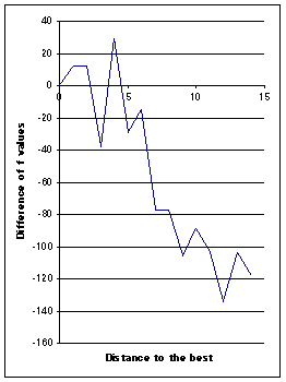
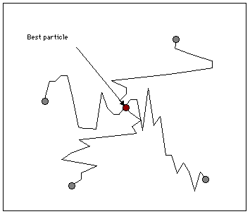
Figure 3. Main sections for a 5-swarm
The landscape is clearly quite chaotic, so we surely will have to use quite often the NoHope/ReHope process. Also, Queens option is probably not efficient.
Let us suppose we know a solution ![]() . We consider all the positions of the search space, an plot the map
. We consider all the positions of the search space, an plot the map ![]() . On this map, at each time step, we highlight the positions of the particles, so that we can see how it moves. We have some equivalence classes according to the equivalence relation
. On this map, at each time step, we highlight the positions of the particles, so that we can see how it moves. We have some equivalence classes according to the equivalence relation ![]() . As we can see, not only is the swarm globally moving towards the solution, but also some particles tend to move towards the minimum (in terms of objective function value) of the equivalence classes. It means that even if it do not find the best solution, it finds at least (and usually quite rapidly) interesting quasi-solutions. It also means that if the swarm is big enough, we may simultaneously find several solutions.
. As we can see, not only is the swarm globally moving towards the solution, but also some particles tend to move towards the minimum (in terms of objective function value) of the equivalence classes. It means that even if it do not find the best solution, it finds at least (and usually quite rapidly) interesting quasi-solutions. It also means that if the swarm is big enough, we may simultaneously find several solutions.
In our example, as the number of positions is quite big (![]() ), we plot only a few selection of them (4700). We use here a swarm size of 16. In Figure 4, we see clearly that the example has been designed to be a bit difficult, for there is a "gap" between distances 4 and 8, but, finally, the swarm finds three solutions in one "standard" run, and some others if we modify the parameters (see Appendix).
), we plot only a few selection of them (4700). We use here a swarm size of 16. In Figure 4, we see clearly that the example has been designed to be a bit difficult, for there is a "gap" between distances 4 and 8, but, finally, the swarm finds three solutions in one "standard" run, and some others if we modify the parameters (see Appendix).
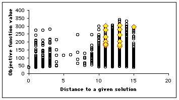
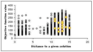
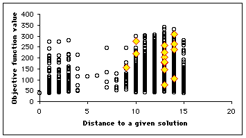
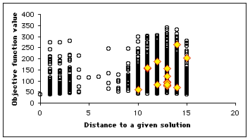
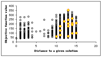
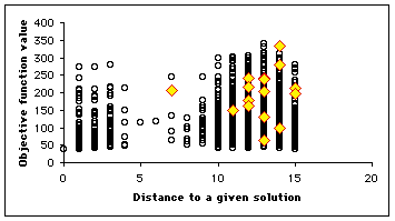
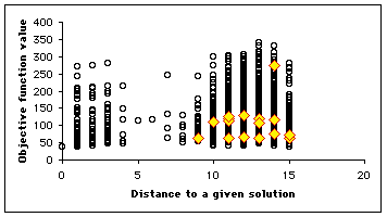
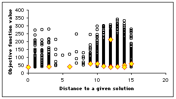
Figure 4. How the swarm moves on the Structured Search Map

Table 1. Some results using Discrete PSO on the graph br17.atsp
|
Swarm size |
Hood size |
c 1 |
Random c2 |
ReHope type |
Best solution |
Hood type |
Tour evaluations |
Arithmetical/logical operations |
|
16 |
4 |
0.5 |
]0,2] |
ADM |
39 (3 solutions) |
social |
7990 |
4.8 M |
|
16 |
4 |
0.5 |
]0,2] |
ADM |
39 |
physical |
7742 |
6.3 M |
|
16 |
4 with queens |
0.5 |
]0,2] |
ADM |
39 (3 solutions) |
social or physical |
9051 |
5.8 M |
|
8 |
4 |
0.5 |
]0,2] |
ADM |
39 |
social |
4701 |
2.8 M |
|
1 |
1 |
0.5 |
]0,2] |
ADM |
44 |
social |
926 to ¥ |
0.6 M |
|
128 |
4 |
0.999 |
]0,2] |
no |
47 |
social |
41837 to ¥ |
33.2 M to ¥ |
|
32 |
4 |
0.999 |
]0,2] |
no |
66 |
social |
14351 to ¥ |
10.8 M to ¥ |
|
16 |
4 |
0.999 |
]0,2] |
no |
86 |
social |
2880 to ¥ |
1.9 M to ¥ |
As we can see on Table 1:
Results are not particularly good nor bad, mainly for we use a generic ReHope method which is not specifically designed for TSP. But this is on purpose: so, by just changing the objective function, you could use Discrete PSO for different problems.
In the original data, diagonal values are equal to 9999. Here, they are equal to 0. For PSO algorithm, it changes nothing, and it simplifies the visualization program.
NAME: br17
TYPE: ATSP
COMMENT: 17_city_problem_(Repetto)_Opt.:_39
DIMENSION: 17
EDGE_WEIGHT_TYPE: EXPLICIT
EDGE_WEIGHT_FORMAT: FULL_MATRIX
EDGE_WEIGHT_SECTION
0 3 5 48 48 8 8 5 5 3 3 0 3 5 8 8 5
3 0 3 48 48 8 8 5 5 0 0 3 0 3 8 8 5
5 3 0 72 72 48 48 24 24 3 3 5 3 0 48 48 24
48 48 74 0 0 6 6 12 12 48 48 48 48 74 6 6 12
48 48 74 0 0 6 6 12 12 48 48 48 48 74 6 6 12
8 8 50 6 6 0 0 8 8 8 8 8 8 50 0 0 8
8 8 50 6 6 0 0 8 8 8 8 8 8 50 0 0 8
5 5 26 12 12 8 8 0 0 5 5 5 5 26 8 8 0
5 5 26 12 12 8 8 0 0 5 5 5 5 26 8 8 0
3 0 3 48 48 8 8 5 5 0 0 3 0 3 8 8 5
3 0 3 48 48 8 8 5 5 0 0 3 0 3 8 8 5
0 3 5 48 48 8 8 5 5 3 3 0 3 5 8 8 5
3 0 3 48 48 8 8 5 5 0 0 3 0 3 8 8 5
5 3 0 72 72 48 48 24 24 3 3 5 3 0 48 48 24
8 8 50 6 6 0 0 8 8 8 8 8 8 50 0 0 8
8 8 50 6 6 0 0 8 8 8 8 8 8 50 0 0 8
5 5 26 12 12 8 8 0 0 5 5 5 5 26 8 8 0
EOF
|
1 |
3 |
14 |
11 |
13 |
2 |
10 |
15 |
7 |
6 |
16 |
4 |
5 |
9 |
17 |
8 |
12 |
1 |
|
1 |
6 |
7 |
15 |
16 |
5 |
4 |
17 |
9 |
8 |
10 |
2 |
13 |
11 |
14 |
3 |
12 |
1 |
|
1 |
7 |
6 |
15 |
16 |
5 |
4 |
9 |
8 |
17 |
10 |
11 |
13 |
2 |
14 |
3 |
12 |
1 |
|
1 |
9 |
8 |
17 |
5 |
4 |
15 |
6 |
7 |
16 |
13 |
10 |
11 |
2 |
3 |
14 |
12 |
1 |
|
1 |
12 |
3 |
14 |
10 |
2 |
13 |
11 |
17 |
8 |
9 |
5 |
4 |
7 |
6 |
16 |
15 |
1 |
|
1 |
12 |
3 |
14 |
10 |
11 |
2 |
13 |
17 |
8 |
9 |
4 |
5 |
16 |
6 |
15 |
7 |
1 |
|
1 |
12 |
6 |
7 |
15 |
16 |
5 |
4 |
9 |
17 |
8 |
2 |
11 |
13 |
10 |
14 |
3 |
1 |
|
1 |
12 |
8 |
9 |
17 |
5 |
4 |
16 |
15 |
7 |
6 |
10 |
2 |
11 |
13 |
14 |
3 |
1 |
|
1 |
12 |
14 |
3 |
2 |
10 |
11 |
13 |
17 |
9 |
8 |
5 |
4 |
15 |
6 |
7 |
16 |
1 |
|
1 |
12 |
14 |
3 |
11 |
2 |
10 |
13 |
15 |
6 |
16 |
7 |
4 |
5 |
9 |
8 |
17 |
1 |
|
1 |
12 |
15 |
16 |
7 |
6 |
5 |
4 |
8 |
17 |
9 |
11 |
10 |
2 |
13 |
14 |
3 |
1 |
|
1 |
12 |
16 |
15 |
7 |
6 |
4 |
5 |
9 |
8 |
17 |
10 |
2 |
11 |
13 |
14 |
3 |
1 |
|
1 |
12 |
16 |
15 |
7 |
6 |
5 |
4 |
8 |
9 |
17 |
10 |
11 |
2 |
13 |
14 |
3 |
1 |
|
1 |
12 |
16 |
7 |
6 |
15 |
5 |
4 |
9 |
17 |
8 |
11 |
10 |
13 |
2 |
14 |
3 |
1 |
|
1 |
12 |
17 |
8 |
9 |
5 |
4 |
15 |
16 |
7 |
6 |
2 |
10 |
11 |
13 |
3 |
14 |
1 |
|
1 |
12 |
17 |
8 |
9 |
5 |
4 |
15 |
16 |
7 |
6 |
2 |
10 |
11 |
13 |
3 |
14 |
1 |
|
1 |
14 |
3 |
10 |
13 |
11 |
2 |
17 |
8 |
9 |
4 |
5 |
15 |
6 |
16 |
7 |
12 |
1 |
|
1 |
14 |
3 |
10 |
13 |
11 |
2 |
8 |
17 |
9 |
4 |
5 |
15 |
6 |
7 |
16 |
12 |
1 |
|
1 |
14 |
3 |
10 |
11 |
2 |
13 |
8 |
17 |
9 |
4 |
5 |
15 |
7 |
6 |
16 |
12 |
1 |
|
1 |
16 |
6 |
7 |
15 |
4 |
5 |
9 |
8 |
17 |
13 |
11 |
10 |
2 |
3 |
14 |
12 |
1 |
|
1 |
16 |
6 |
7 |
15 |
4 |
5 |
9 |
8 |
17 |
13 |
10 |
2 |
11 |
3 |
14 |
12 |
1 |
|
1 |
17 |
9 |
8 |
4 |
5 |
7 |
6 |
16 |
15 |
10 |
11 |
2 |
13 |
14 |
3 |
12 |
1 |
|
1 |
12 |
14 |
3 |
2 |
10 |
13 |
11 |
16 |
6 |
7 |
15 |
4 |
5 |
17 |
9 |
8 |
1 |