Mathematical form of the problem and convergence cost
For simplicity the space of search is an hypercube ![]() on wich is defined an objective function f. We are looking for a point
on wich is defined an objective function f. We are looking for a point ![]() so that, for a given objective value S and a given acceptable error value
so that, for a given objective value S and a given acceptable error value
For a given swarm size N, and a given iterative algorithm A the problem is to evaluate the "cost" of a solution. This "cost" is often definedjust as the number of time steps T neededbut we define here a more realistic one, depending on the swarm size N, on the probability ![]() to have a solution in at most T time steps and on the wanted probability of success
to have a solution in at most T time steps and on the wanted probability of success ![]() . The basic idea is that if we want to reach the probability
. The basic idea is that if we want to reach the probability ![]() , we have to try tT " times " for the N particles, where t is given by
, we have to try tT " times " for the N particles, where t is given by
|
|
Equation 1 |
So our cost is defined as follow
|
|
(for continuity reason, we also define $A=NT if ![]() and
and ![]() are equal to 1).
are equal to 1).
The Most Stupid Algorithm
At each time step, we choose N positions xi completely at random (uniform distribution) in the hypercube, and we check if, by chance, at least one of them is a solution.
Estimation of the probability of success for one particle
If the function f is simple enough, we can directly compute ![]() , that is to say a measure of the size of the solution set. By dividing by
, that is to say a measure of the size of the solution set. By dividing by ![]() , we find the exact value of
, we find the exact value of ![]() . This is the probability to find immediately (T=1) a solution, by chance, and we will simply call it
. This is the probability to find immediately (T=1) a solution, by chance, and we will simply call it ![]() .
.
Example

Then we have
![]()
Now, if we don't find immediately a solution, we can choose another position at random, and so on. The probability to find (at last !) a solution at the time step T (and not before) is ![]() .
.
So the probability the find a solution at T or before is
We can also retrieve this formula by observing that the probabilitywe are looking for can be described as "the opposite of the case where no solution is found at T or before".
Example
With the same values as in the previous example, we obtain the following curve:

Figure 1. Probability of immediate success by chance for one particle.
But usually the objective function is not simple, and we can just have an estimation of ![]() : for instance we can try, at random, a lot Lof x points, and count the number of successes l. The estimation is then
: for instance we can try, at random, a lot Lof x points, and count the number of successes l. The estimation is then ![]() .
.
Example
Still with the same example, we have:

Figure 2. Preliminary test to estimate the probability of immediate success.
Estimation of the probability of success for N particles
Either by direct calculus or by statistical estimation as aseen above, we suppose we have a value for p0, so that we can compute ![]() .
.
Now, if we increase the number of particles, it is clear we increase our chance to find a solution. In fact, we have the relation
|
|
This formula comes from the fact that all attempts are completely independent. So, what it is important is just the total number NT of random positions. But it is interesting to not that the cost, as defined above, is completely independent on NT. We have indeed, by combining Equation 2, Equation 3 and Equation 4
![]()
In particulat, if ![]() we obtain an infinite cost : we cannot be completely sure to reach the objective.
we obtain an infinite cost : we cannot be completely sure to reach the objective.
Example
Still for ![]() , this relation gives us the possibility to plot some interesting curves, for example how increases the probability of success with N (and T) or how decreases the time needed for success with the swarm size (for a given probability).
, this relation gives us the possibility to plot some interesting curves, for example how increases the probability of success with N (and T) or how decreases the time needed for success with the swarm size (for a given probability).

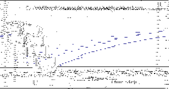
Figure 3. MSA: Probability of success vs Swarm size.

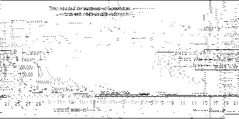
Figure 4. MSA: Time for success vs Swarm size.
Maurice.Clerc@WriteMe.com 1998/11/23