Discrete Particle Swarm Optimization: A Fuzzy Combinatorial Black Box
Maurice.Clerc@WriteMe.com2000/04/28
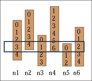
A small Fifty-fifty example
Figure 2. A Fifty-fifty example.
Let ![]() be six finite lists of different integer numbers. Let
be six finite lists of different integer numbers. Let ![]() be the j-th value in the list
be the j-th value in the list ![]() . We want to find six such values, all different, so that we have
. We want to find six such values, all different, so that we have ![]() . This example is an adaptation of the one you can find in . In particular, I have added the condition "all different", so that the problem is a bit more difficult.
. This example is an adaptation of the one you can find in . In particular, I have added the condition "all different", so that the problem is a bit more difficult.
Implicit Search Space
The Implicit Search Space is simply the list of the lists. Here, it is defined as
((0,1,2,3,4),(0,1,2,3,4),(0,1,2,3),(1,2,3,4,5,6),(0,1,2),(0,1,2,3,4))
If ![]() is the length of the list
is the length of the list ![]() , the ISS generates the real search space which size is
, the ISS generates the real search space which size is ![]() , (9000 here).
, (9000 here).
Crisp representation
Position and velocity
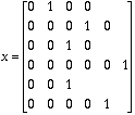
A "position" x is a list of 6 possibles values, the i-th value is chosen in ![]() .
.
Example: x=(1,3,2,6,2,4)
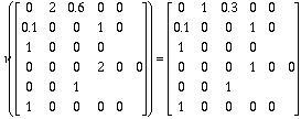
A "velocity" is an operator which, applied to a position, and calculated by a given algorithm, gives another position.
Example: ![]()
The condition " calculated by a given algorithm" is necessary, for two velocities can be equivalent, and there is not necessary juste one "smallest" one.
Note that if we apply, say ![]() , to a value different from 0, nothing happens.
, to a value different from 0, nothing happens.
The size of a velocity, ![]() , is tne number of components which are not equivalent to "do nothing", (like
, is tne number of components which are not equivalent to "do nothing", (like ![]() ). In the above example, the size is 5.
). In the above example, the size is 5.
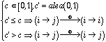
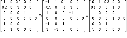
Operators for PSO equations
We use here the system
![]()
Equation 1. Moving a given particule.
where ![]() is the best previous position of the particule and
is the best previous position of the particule and ![]() the best previous position in the neighbourhood (eventually the whole swarm). The four operators needed are
the best previous position in the neighbourhood (eventually the whole swarm). The four operators needed are
coeff_times_vel (![]() ) : = (real positive coefficient, velocity) ®
velocity
) : = (real positive coefficient, velocity) ®
velocity
vel_plus_vel (![]() ) := (velocity, velocity) ®
velocity
) := (velocity, velocity) ®
velocity
pos_minuspos (![]() ) := (position, position) ®
velocity
) := (position, position) ®
velocity
pos_plus_vel (![]() ) := (position, velocity) ®
position
) := (position, velocity) ®
position
Figure 2 is self explanatory, except maybe for coeff_times_vel.
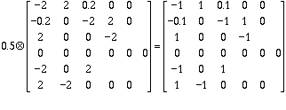
Note that the operator coeff_times_vel is stochastic, and defined only for a coefficient between 0 and 1. For a coefficient greater than 1, say coeff=k+c, with k integer and c<1, we can simply use k times vel_plus_vel and one times coeff_times_vel with c.
Here is how coeff_times_vel is computed for a coefficient c:
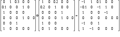
Note also that vel_plus_vel is not commutative. In the algorithm I have written, it seems the best way is to add velocities in increasing order (of size).
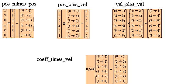
Figure 3. The four operators for a crisp combinatorial black box (examples).
Cost function
As usually, there are an infinity of possible cost function to minimize. Of course, the simplest one is, as always, a binary good/no good function:
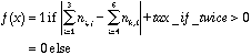
but convergence is obviously difficult with such an almost non discriminatory function, so I use the more reasonable one:
![]()
where tax_if_twice is simply the greatest value in the ISS (6, here).
Example:
![]()
It works but…
The main parameters are
Swarm size s
Neighbourhood size h
Social/cognitive confidence coefficients c1, c2, c3.
A swarm size just equal to the maximum length of the ni lists and a neighbourhood size just equal to 5 seems to give always the best results. Let us consider what happens when we modifiy confidence coefficients (Performance Map). Note that, as usually, a NoHope/ReHope is used to reach exactly a solution and not only an approximation.
As we can see on the Figure 3, which shows the number of cost evaluations to reach a solution, it is quite difficult to find good coefficients, for we have mainly very bad results. On the other hand (but the map is not detailed enough to see it), for some rare parameters values, we have quite good performances (about 100 evaluations).
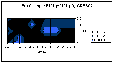
Figure 4. A Performance Map for Crisp Discrete PSO.
For example, for the coefficients (c1=0.3, c2=c3=4), a solution is found after 102 evaluations of the cost function. As there are 8 solutions among 9000 positions, the probability to obtain this result just by chance is about 8.7% ![]() . We find more or less the same probability with bigger examples. It seems not that bad, but in fact it is, for at least two reasons:
. We find more or less the same probability with bigger examples. It seems not that bad, but in fact it is, for at least two reasons:
In practice, it means we have to try different possible sets, so, the true number of evaluations may be far bigger, typically 1000, which is very bad (probability to find it just by chance=60%). And we have to do that for the algorithm is not very "robust": even a small change in confidence coefficients may give a far better or far worse result. That is why it seems a good idea to use a fuzzy representation, for it is well known fuzzy algorithms are usually very robust.
Fuzzy representation
Position and velocity
Each component of the position is now not only a single number, but a fuzzy set on the possible values, that is to say, for the i-th component, a set of ![]() confidence coefficients on [0,1] (note that these "confidence coefficients" have nothing to do with the social/cognitive confidence coefficients ck in Equation 1.
confidence coefficients on [0,1] (note that these "confidence coefficients" have nothing to do with the social/cognitive confidence coefficients ck in Equation 1.
For example, the position (1,3,2,6,2,4) would be now, reffering to the ISS
((0,1,2,3,4),(0,1,2,3,4),(0,1,2,3),(1,2,3,4,5,6),(0,1,2),(0,1,2,3,4)),
The good point is that we can now move more "continuously", for intermediate positions are defined, as soon as some coefficients are between 0 and 1 (see examples below). Another interesting point is that a "velocity" has exactly the same representation than a position: a list of fuzzy sets. The only difference is that the coefficients can have any real value (not only on [0,1]). It gives us a very natural way to define the operators, in particular coeff_times_vel.
Operators
We need two additional operators:
normalize ( ![]() ) := (fuzzy position) ®
(fuzzy position)
) := (fuzzy position) ®
(fuzzy position)
defuzz ( ![]() ) := (fuzzy position) ®
(crisp position)
) := (fuzzy position) ®
(crisp position)
We apply "normalize" to be sure all coefficients in a fuzzy position are in [0,1], and "defuzz" to obtain a crisp position on which the cost function can be calculated as before. The examples below show how the operators work (remember that the coefficients are reffering to the ISS).
normalize
defuzz

pos_minus_pos
pos_plus_vel
vel_plus_vel
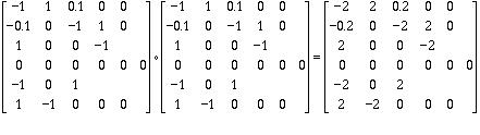
coeff_times_vel
Cost function
We apply exactly the same cost function, but to the "defuzzified" position ![]()
Results
As expected, the algorithm is now very robust: the number of cost evaluations is almost the same on a large range of parameters (see Figure 4).
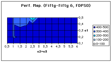
Figure 5. A performance map for Fuzzy Discrete PSO.
Of course this number (about 400) is still far too high for it means the probability to have found a solution just by chance is about 30%. But this is for one run. The probability to find a solution just by chance in less than 400 evaluations for r consecutive runs (with coefficients randomly chosen) is rapidly decreasing with r. And, more important, the probability to have to perform more than 500 evaluations to find a solution is simply equal to zero.
Temporary conclusion
So it seems it is really worthwhile to use fuzzy representations, when we have no way to "guess" efficiently what could be the best parameters: at least, we are sure to not obtain results worse than a pure random or exhaustive search as sometimes with crisp representations! Now, there are of course two questions:
References