Algebraic view

The basic simplified dynamic system is defined by
 

Equ. 1

where .

Let  be the current point in , and  the matrix of the system. So we have  and, more generally, 

So the system is completely defined by M.

The eigenvalues of M are:
 

Equ. 2

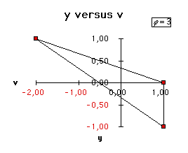
We see immediately that the value j=4 is special. We will see below what it means.

For j # 4 we can define a matrix A so that 

(if j =4, A^-1 doesn’t exist).

For example, from the canonical form  we find

In order to have simpler formulas, we can multiply by 2j, to produce a matrix A:

So if we define  we can now write

that is to say we have, finally, 

But L is a diagonal matrix, so we have simply 

In particular, we have a cyclic behavior if and only if  (or, more generally if ). This just means that we have the system of two equations:

Case j<4

For j<4, the eigenvalues are complex, and there is always at least one (real) solution for j.

More precisely we can write

with  and 

and then

and cycles are given by any q so that 

So for each t, the solutions for j are given by

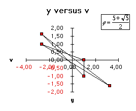
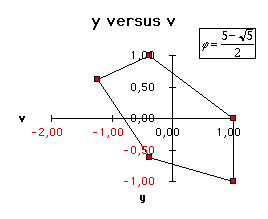
Table 1 gives some nontrivial values of j for which the system is cyclic.
 

j	size of the cycle
3	3 (see Figure 1)
2	4
	5 (see Figure 2 and Figure 3)
1, 3	6,3
1, 2, 3,	6, 4, 3, 12

For any other value, the system is just quasi-cyclic (see Figure 4).

We can be a little bit more precise. Below,  is the 2-norm (the Euclidean one for a vector).

We have here

For example, for v₀=0 and y₀=1, we have

Figure 1. 3-cycle.

Figure 2. Non convex 5-cycle.

Figure 3. Convex 5-cycle.

Figure 4. Quasi-cycle.

Case j>4
 
 

If j>4, then e₁ and e₂ are real numbers (and ), so we have either

• (for t even) which implies j=0, not consistent with the hypothesis j>4
• (or -1) which is impossible
• 

So, and this is the point, there is no cyclic behavior for j>4. And, in fact, the distance from the point  to the center (0,0) is strictly increasing with t.
 
 

We have

So

But we can also write

So, finally, is increasing "like".

This result can be used to prevent the "explosion" of the system by defining "constriction" coefficients.

Case j=4

We have here 

In this particular case, the eigenvalues are both equal to -1, and there is just one family of eigenvectors, generated by . So we have .

So, if P₀ is an eigenvector, proportional to V (that is to say if ), we just have two "symmetrical" points, for

In the case where P₀ is not an eigenvector, we compute directly how  is decreasing and/or increasing. Let us define .

It is easy to see (by recurrence) we have has the following form:

where a_t,b_t,c_t are integer numbers so that  for .

Now, let’s suppose for a particular t we have . What about  ?

We easily compute .

This quantity is positive if and only if v_t is not between (or equal to) the roots 

Now, if we compute  we have, and the roots are. As , it means that  is also positive.

So as soon as  begins to increase, it does so infinitely.

But it can be decreasing, at the beginning. How many times ?

Suppose we have D₀ < 0.

It means v₀ is between -2y₀ and -12y₀. For instance in the case y₀>0, we can write

, with 

By recurrence, we have then

, with 

Finally, we can write

as long as

that is to say (for t is an integer) as long as

After that, increases.

We can do exactly the same analysis for y₀<0. In this case e<0 too, so the formula is the same.

In fact, we can even be more precise. If we define

then we have

That is to say  is decreasing/increasing almost linearly when t is big enough. In particular, even if it begins to decreases, after that it tends to increase almost like .